gait variability

Electing a representative

One of the aspects of gait analysis that I didn’t cover in any particular depth in my book was how to select data from a number of trials that is in someway representative of the patient. I think one of the reasons for this is because I couldn’t easily get my hands on any data that illustrated the issues well. In some ways this speaks for itself – in my experience large inter-trial variability, larger enough to affect how we interpret data, is actually quite rare in clinical practice. If the variability is small then it doesn’t really matter what technique you choose.

representative-trial

My personal preference is to avoid the issue altogether by overplotting data from multiple trials on the same graphs (similar to the graphs on the left above but with data from the other side plotted in a different colour as well). In this way you can take into account both the general pattern and the variability when interpreting the data. Some people object that using this technique it can be difficult to appreciate subtle features in individual traces, but there is a real question as to whether you should be even looking at such features if they are not consistent from trace to trace.

Now I’ve started annotating graphs with symbols to identify specific features in the data, however, I find that the combination of symbols and multiple curves can be a bit too messy and have resorted to looking to a single trace that can be taken of as representative. Although alternatives have been proposed I use the average trace. It leads to a little smoothing of the data – which isn’t perfect – but none of the other techniques are perfect either. It was interesting last week to come across a patient’s data that illustrated beautifully the problems of doing this.

You can see the knee and hip traces here with the individual traces overlaid on the left and the averaged data plotted on the right. The problem is with the left knee. You can see that the patient exhibits two distinct patterns of knee movement in early stance (but remarkable repeatability elsewhere in the gait cycle). She either walks with full knee extension in early stance or with quite marked knee flexion. In the fully extended pattern her knee is more posterior and so there is increased hip extension as well (there is an effect on ankle dorsiflexion as well which I haven’t plotted). The average trace for the knee, however, falls well within normal limits and if you only ever looked at that trace you would never know that there was anything wrong with the knee.

None of the methods that are commonly used to generate a representative trace whether they be through picking one particular trace or providing some sort of averaging (mean or median) will result in something that represents the patient. The fundamental reason these don’t work is that this person’s gait is not characterised by one gait pattern, but by two, which she alternates between. It is not possible to understand her walking on a single curve, you need to look at multiple trials.

So although such issues don’t arise very often we don’t have a good way dealing with them in how we plot out or mark-up our data. What is needed is not a way of selecting single trace but a means of indicating that any single trace is unrepresentative. The broad semi-transparent bands on the right hand graphs are supposed to indicate that the trace cannot be appropriately interpreted without referring to the multiple trial data. I’ve now added them to the list of symbols that we use for marking up our graphs.

(PS The idea for a symbol to indicate underlying variability in the multiple trial data was first suggested to me by Sheila Gibbs in Dundee during an early consultation on the Impairment Focussed Interpretation methodology I outline in my book.)

(PPS if you do feel a need to select a representative trace and want to do this systematically then a robust method is presented by Morgan Sangeux in this recent paper. It is however worth noting that in the example he gives in Figure 1 the trace chosen as most representative overall does not give a good indication of the underlying data for either pelvic tilt or foot rotation despite the rigour of the technique.)

Advertisement

Normalising kinetics

There were a few things that struck me as odd when I was writing my book. Things that we’ve always done in a particular way in clinical gait analysis but which just don’t make sense. One of these is the way we typically “normalise” kinetic data by dividing through by mass only. Moments are a product of force and length and are thus likely to be influenced both by a person’s weight and their size. It just doesn’t make sense to normalise data by dividing through by weight only. There are similar, but slightly more complex, issues with joint power. Differences in adult height between individuals, expressed as a percentage, tend to be reasonably small (SD < 10%) even disregarding gender, so the effects of not normalising to height in adults are unlikely to be that important. Clinical gait analysis, however, has always had a considerable focus on children where differences in height are much larger. It just seems so obvious that we should normalise to height as well as weight. In my book I see that I actually commented, “Quite why this is not standard practice in gait analysis is unclear.”

A simple explanation may be that no-one has ever tested this assumption. So one of my colleagues (Ornella Pinzone) has performed a comparison of conventional normalisation (dividing moments and powers by mass only) and non-dimensional normalisation (dividing moments by mass and leg length and powers using a slightly more complex formula). We based it on data made available by Mike Schwartz from Gillette as their data are so well formatted for a study like this. The paper has just been published in Gait and Posture and if you use this link before 29th January then you should be able to view and download a copy of the article for free.

Pinzone

Coefficients of determination for relationship between a range of temporal, spatial and kinetic parameters and age amongst children across an age range from 4 to 18 years. Dashed line shows threshold for statistical significance at p<0.05.

The results are quite conclusive. About 80% of the associations between the conventionally normalised parameters and age, height and weight, were statistically significant (p<0.05) and for all of those parameters where the association was significant it was substantially reduced by non-dimensional normalisation (only just over 20% were statistically significant and most only marginally exceeded the p<0.05 threshold). The results have dispelled any lingering doubts in my mind as to the superiority of non-dimensional normalisation and when we next revise our normative dataset we’ll be using this as standard.

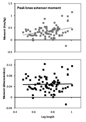
This isn’t quite the whole story, however, because even when you remove the systematic effects of height and weight (this is the primary purpose of normalisation) there is still a lot of scatter in the data. The figure below shows the relationship of peak knee extensor moment with leg length for conventional (top) and non-dimensional (bottom) normalisation. The slope on the line of regression is reduced to almost zero with non-dimensional normalisation but there is minimal effect on the scatter of data points about this line.

Pinzone2

Peak knee extensor moment plotted against leg length for conventional (top) and non-dimensional (bottom) normalisation.

It is difficult to compare this variability with that present in kinematic data because the nature of the data is so different but the impression I get is that the variability in the kinetic data is even greater than that in the kinematic data. I’ve commented in two earlier posts (here and here) that I think the assumption that we all walk similarly, an assumption on which all clinical gait analysis is based, needs to be re-examined. The most obvious conclusion from this dataset is that many of us, even in the absence of pathology, walk very differently.

I know her by her gait

Thinking about the range of variation there is within “normal” walking last week has reminded me of a couple of studies that exemplify this.

Male and female walking

One of the nicest and most fun is from Niko Troje‘s Biomotion lab group at Queen’s University in Kingston, Ontario. Niko recorded the movement of retro-reflective markers on 20 men and 20 women and used a principal component analysis to analyse the data in such a way that it was possible to define the characteristics that differed with gender. He then used this information to to synthesise archetypal movement patterns for males and females. What makes it great fun is that he’s produced a flash demonstration  of this called BMLwalker that allows you to adjust the gender balance and see how the gait pattern changes (click on the picture below, the animation will open in a new tab, and  you can then play with the male/female slider). He also had the people’s weights so you can play with a slider which effectively adjusts the weight of the synthetic person you are looking at.

BMLwalker

In a novel twist Niko then got people to rate the movement patterns on a scale of sad to happy and nervous to relaxed and used the information to create sliders for these as well. The system works in such a way that you can mix these and look at the archetypal gait pattern of a relaxed but sad heavy male if you want to.

The important part of this (for me) is of course that it is all based on an analysis of the variability within the “normal” range of walking patterns (do note that the technique allows for the synthesis of ultra-archetypes that are beyond the normal range but only on the basis of an analysis of the variability within gait patterns that were originally within that range)

Muggability

I’m also reminded of the classic study from the 1980s in which  Grayson and Morris took essentially anonymised videos of 60 individuals and showed these to 53 criminals in a local prison for a range of offences from assault to murder. They asked them which looked more vulnerable and who they might be more likely to mug given the choice. There was reasonable agreement amongst the criminals. About 20 years later Gunns, Johnston and Hudson repeated the work but this time using a point light representation similar to that in the flash animation that you’ve just looked at. They found that vulnerability could be assessed on the pattern of moving lights alone. This demonstrates once again that within the normal range of walking patterns there is considerable variability.

It is actually possible to do this study for yourself because if you look more closely at BMLwalker you’ll see a more button. If you click this then the software will present you with a large number of gait patterns and allow you to grade each one on any scale. I’ve typed in muggability and graded the patterns by whether I think they they look confident and assertive or timid and weak. I graded about 50 patterns (you  just press End experiment when you’ve had enough)  and the software calculated a slider to adjust for muggability. I didn’t think I was doing all that well but when I looked at the results they were really convincing. Try it for yourself and see what you think.

Sex appeal

And here’s a video I just happened to come across while searching the web to find the BMLwalker. I’ll let you judge whether, despite the title, you thinks its science or not!

Video from the Discovery Channel’s Science of Sex Appeal (2009)