normal walking

More on muscle

In his comment to my last post BJ said, “I think our field needs some general physiological principles (such as “muscles generate very little passive force during walking”) to help improve the accuracy of our muscle force estimation process”. In his book Rick Lieber states, ” It is difficult to hypothesise, a priori, the ‘best’ sarcomere length operating range of muscle”. So there’s a challenge!

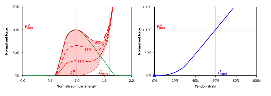
In looking at the issues I realise that I’ve never really seen a simple analysis of how a muscle and tendon work together in series (most I’ve looked at get very complicated very quickly, e.g Winters as quoted by Thelen). So let’s take the well known properties of the force length curves for muscle and tendon (see Figures below) and try and consider how they would lead a simple musculotendinous unit to behave.

Muscle and tendon

Let’s assume the simplest possible arrangement of these as two elements in series held at fixed length. Let’s start off by analysing what happens when this fixed length is what I call musculotendinous unit slack length. This is the minimum separation of origin and insertion at which both the inactive muscle and tendon generate no tension (muscle at optimal length, tendon at tendon slack length to use the jargon).

MTU

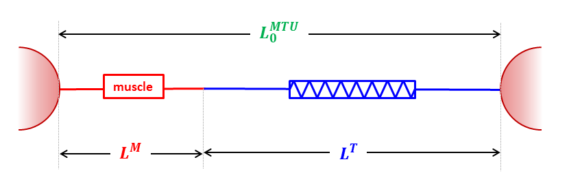
Its obvious that together the length of the muscle and tendon must equal the fixed length we’ve chosen so it becomes possible to plot the force generated in the tendon as a function of muscle length on the same graph as that for the muscle (see Figure below). It looks steeper because the horizontal scales of the two graphs above are different and it appears to be the wrong way round because as the muscle get’s longer the tendon will get shorter.

MTU graph

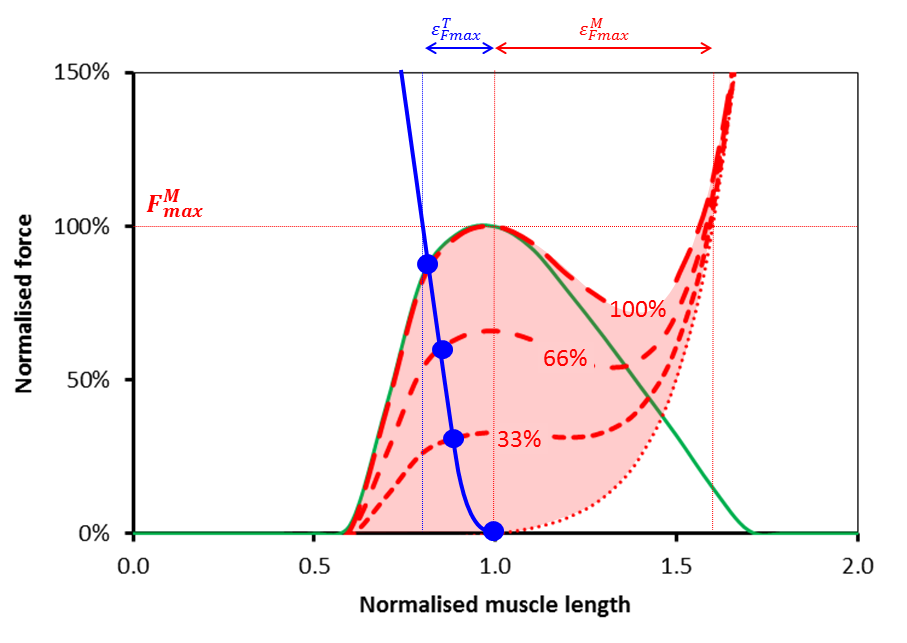
Now if any two mechanical elements are in series like this we know that the same force must pass through both (these are the laws of physics and we can’t do anything about them). We can thus say that the force generated by the musculotendinous unit as a whole must be equal to that at the point at which the red line and the blue lines cross for a given level of activation (represented by the blue dots for 0, 33%, 66% and full activation). You’ll see that as the muscle get’s more activated this point moves up and to the left. The tension in the musculotendinous unit increases as the muscle shortens (and hence the tendon lengthens) which is what you would expect.

Notice however that the force must lie somewhere on the blue curve. This restricts quite severely the range of muscle lengths at which the musculotendinous can generate force. Rather counter-intuitively (at least to my simple mind) the operating length of the muscle as a component of the musculotendious unit appears to be more dependent on the force-length characteristics of the tendon than those of the muscle. Notice also that the maximum force that the unit can generate (the point at which the blue line and maximum activation curve for the muscle intersect) is less than that for the muscle acting in isolation.

At musculotendinous unit lengths the only change in the graph is that the blue line will move to the right (if the unit gets longer) or to the left (if the unit gets shorter). An interesting observation here is that if the blue curve moves too far to the right then there will come a point at which there is a minimum force that the unit can generate as well as a maximum. This makes sense in that if you stretch the musculotendinous unit too far you will be stretching the passive parallel component in the muscle regardless of whether it is activated or not.

But let’s take that in combination with the observation I focussed on in last week’s post that when we move the joints passively (through much more than the  range of movement required for walking) during a physical examination of a healthy adult we encounter minimal resistance. This suggests that there must be a limit to how far to the right that blue line can be during walking. If we assume the resistance to passive stretch over the range of movement required for walking is less than 5% of the maximum force that the muscle can generate isometrically (I think this is quite a reasonable constraint to impose) then the most right-ward position of the solid blue line is that illustrated in the figure below. You can see that this restricts the operating range of the muscle even more than the logic I applied last week. Last week I argued that the muscle cannot be operating on the passive arm of the the force-length curve.  This week I’m suggesting that it cannot be operating on much of the descending arm either.

MTU graph (max)

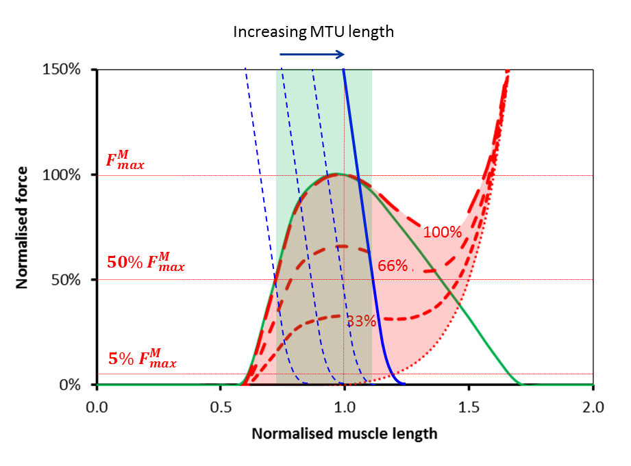
The thinner dashed curves show the behaviour of the system when the musculotendinous unit is shorter. As well as a line at 5% of maximum muscle force I’ve drawn another in at 50%.  The green region is thus intended to show the range of muscle lengths over which the musculotendinous unit is capable of generating this level of force. It suggests that in order for effective force generation by the musculotendinous unit the muscle lengths must lie between about 70% and 110% of optimum length.

The curves, particularly that for tendon, will vary from muscle to muscle (and maybe from individual to individual). The data illustrated here are those use to describe the lateral gastrocnemius in the Gait2392 model which is available through the OpenSim web-site (although I’ve tweaked the characteristics of active muscle force generation to match the widely accepted work of Gordon et al.). I’ve tried it with a semimembranosus as well and get a slightly steeper tendon curve (when scaled to optimum muscle length) but broadly the same conclusions. The analysis assumes isometric contractions of the muscle but given that most of the conclusions are dependent on the characteristics of the force-length curve for tendon rather than that for muscle I can’t see how consideration of the force-velocity characteristics of muscle can make that much difference.

I’d be particularly interested to know if anyone has seen a similar analysis in print anywhere. Have I just been looking in the wrong places?


Advertisement

I know her by her gait

Thinking about the range of variation there is within “normal” walking last week has reminded me of a couple of studies that exemplify this.

Male and female walking

One of the nicest and most fun is from Niko Troje‘s Biomotion lab group at Queen’s University in Kingston, Ontario. Niko recorded the movement of retro-reflective markers on 20 men and 20 women and used a principal component analysis to analyse the data in such a way that it was possible to define the characteristics that differed with gender. He then used this information to to synthesise archetypal movement patterns for males and females. What makes it great fun is that he’s produced a flash demonstration  of this called BMLwalker that allows you to adjust the gender balance and see how the gait pattern changes (click on the picture below, the animation will open in a new tab, and  you can then play with the male/female slider). He also had the people’s weights so you can play with a slider which effectively adjusts the weight of the synthetic person you are looking at.

BMLwalker

In a novel twist Niko then got people to rate the movement patterns on a scale of sad to happy and nervous to relaxed and used the information to create sliders for these as well. The system works in such a way that you can mix these and look at the archetypal gait pattern of a relaxed but sad heavy male if you want to.

The important part of this (for me) is of course that it is all based on an analysis of the variability within the “normal” range of walking patterns (do note that the technique allows for the synthesis of ultra-archetypes that are beyond the normal range but only on the basis of an analysis of the variability within gait patterns that were originally within that range)

Muggability

I’m also reminded of the classic study from the 1980s in which  Grayson and Morris took essentially anonymised videos of 60 individuals and showed these to 53 criminals in a local prison for a range of offences from assault to murder. They asked them which looked more vulnerable and who they might be more likely to mug given the choice. There was reasonable agreement amongst the criminals. About 20 years later Gunns, Johnston and Hudson repeated the work but this time using a point light representation similar to that in the flash animation that you’ve just looked at. They found that vulnerability could be assessed on the pattern of moving lights alone. This demonstrates once again that within the normal range of walking patterns there is considerable variability.

It is actually possible to do this study for yourself because if you look more closely at BMLwalker you’ll see a more button. If you click this then the software will present you with a large number of gait patterns and allow you to grade each one on any scale. I’ve typed in muggability and graded the patterns by whether I think they they look confident and assertive or timid and weak. I graded about 50 patterns (you  just press End experiment when you’ve had enough)  and the software calculated a slider to adjust for muggability. I didn’t think I was doing all that well but when I looked at the results they were really convincing. Try it for yourself and see what you think.

Sex appeal

And here’s a video I just happened to come across while searching the web to find the BMLwalker. I’ll let you judge whether, despite the title, you thinks its science or not!

Video from the Discovery Channel’s Science of Sex Appeal (2009)


I know him by his gait

I was asked to be an expert witness for a court case last week. There was some video footage from a CCTV camera of an individual walking across a street from some distance away and the question I was being asked to provide an opinion on was, “Is it possible to identify the individual on the basis of his gait pattern?“.

There are, of course a number of University departments working on related issues (that within Computer Vision at the University of Southampton is a good example) and some evidence of commercial interest.  Every so often the concept bubbles into the popular science magazines. (There is now even an Android app that claims to be able to identify a person from the accelerometer data from a smartphone carried in their pocket while they are walking, but that’s another story).

I’ve generally been rather dismissive of these claims. I strip people down to a pair of shorts, stick retro-reflective markers over anatomical landmarks, ask the person to move in a particular fashion along a clearly marked walkway and then capture the movements with ten extremely high resolution cameras pointing directly at them. It often amazes me how little evidence there is of difference from normative reference data even for individuals with quite marked pathology. If I can’t detect such clear differences under such standardised conditions using such specialised equipment how can anyone suggest that they can recognise a healthy  individual, presumably with a gait pattern within the normal range, on the basis of a video image of them walking down the street fully clothed?

And yet in Shakespeare’s Julius Caesar, Cassius says to Casca when he sees a figure approaching, “Tis Cinna. I do know him by his gait“.  In Melbourne my office was by a corridor and it was generally possible to identify which of my colleagues was approaching along it by the sound of their footsteps. Our common experience is that we do recognise people at least partly by their gait. If gait patterns are so characteristic why is it so difficult to pick up abnormality in clinical gait analysis.

I suspect the answer is partly that gait is so varied and  characteristic. There is much more variability in normal walking than we appreciate. The creation myth of clinical gait analysis is that there is a well-defined pattern of normal walking and that our patients exhibit patterns that differ from this. The longer I think about this idea the less I believe it is true. When we tidy up our normative data by only plotting one standard deviation limits we get reasonably tight normal ranges but this is at the expense of excluding a third of the data (the +/- 1 SD limits only include 67% of the data by definition). If we plot two standard deviations, which represent 95% of the data, then we get much larger bars. Maximum knee extension in stance, for example varies between 5° of hyperextension and 18° of flexion across the healthy population (see figure below).

Knee 2 sd

The reason why it is so difficult to identify gait abnormality among our patients is at least partly because the normal variability between individuals is so large. Maybe on this basis gait as a biometric identifier is not quite so fanciful (although I still have reservations as to whether it will ever work on the basis of CCTV footage recorded in town centres or airports). Perhaps more importantly,  should be studying the characteristics of inter-person variation in gait patterns more closely in order to understand normal walking. In amongst all that variability are there specific characteristics that are invariant? If there are what does that tell us about the requirements of healthy walking? Gait variability within individuals is now seen as providing information about stability and by extension to falls risk (e.g. Callisaya et al. 2011). Maybe we should be paying more attention to gait variability between individuals.

PS Of course the other important factor in recognising people by their gait in every day life is the wide range of information we use to do so. When I recognised people by their footsteps from my office it was probably more to do with the sound that different footwear made as it was to do with temporal-spatial characteristics. One particularly famous CP surgeon was easily identifiable – partly from a mild asymmetry in his footfall pattern but more importantly from the characteristic jangle of coins and or keys in his pocket.

Do it yourself normative data comparison (free download!)

Hi, I’ve had a bit of a break over the summer but I’m hoping to start posting again regularly form now on. Just a reminder that we are running another gait course in November (this one focussing on measurement issues rather than clinical interpretation). Click on the image to the right for more details. There is also just about time to register to start our Masters in Clinical Gait Analysis by distance learning (you don’t need to come to Salford at all). Click on the other image to the right for more details of it.

Enough of the ads, this blog following on from one I wrote just after the GCMAS meeting last year. It had a video link to the presentation I’d just delivered arguing that the reason we collect normative data should be so that we can compare it with other people’s normative data. I presented data showing that if we did that for the normative data from the Royal Children’s Hospital in Melbourne and Gillette Children’s Speciality Healthcare then we get quite remarkable agreement. You can see the comparative kinematic data in the figure below.

compare norms

The paper based on that presentation has finally got published in Gait and Posture (if you don’t have access to the journal you can find a pre-publication version here). We’ve also prepared an Excel file that contains the data in a format that allows you to add your own normative data (mean and standard deviation) to allow comparison with the data from Melbourne and Gillette. Just cut and paste your data into the spreadsheet and look at the graphs to see how you compare. Remember that differences in the mean traces suggest that there are systematic differences in how you apply markers, differences in standard deviations are likely to reflect how consistently you apply them within your own lab.

Do let me know how well your data compares. It might be interesting to post some examples of how various clinical centres compare on this blog-site somewhere.

Swing low

Whenever I give my “Why we walk the way we do” lecture as I did again last week at our gait course (click here to read some of the delegates comments from the Course Evaluation Forms) it makes me think in more detail of some of the biomechanics. This time it made me think more about the swing phase pendulum. In a sense this mechanism is too obvious and we perhaps don’t think enough about it.

There is a historical perspective. The Weber brothers, writing in 1836, assumed a simple pendulum action and came up with a lot of calculations based on elementary physics to support their assumption. Shortly afterwards, however, Guillame Duchenne, noted that he had several patients with isolated flaccid paralysis of the hip flexors who had to walk with circumduction to clear their limb. This suggested an active rather than passive mechanism. It was this question that drove the amazing work of Braune and Fischer in the late 19th century. They confirmed Duchenne’s clinical observation that initiation of swing is an active process.

moments hip

In my lecture I gloss over this a bit leaving the assumption that the pendulum motion during swing is an energy conserving process. It struck me this year that an indication of whether this is the case is to look at the hip moment.  A good definition of a simple, energy conserving pendulum is one in which no moment is exerted at the pivot (hip). Looking at the hip moment  (above, taken from the notes I prepared for the course) it appears to have three phases in swing. In early swing a marked hip flexor moment is exerted accelerating the limb, through middle swing the moment is essentially zero (we do have a simple pendulum movement) and in late swing the hip extensors are active to decelerate the limb.

In a paper that I’ve only just discovered, Holt et al. (1990) do some calculations to estimate natural frequency of the lower extremity and suggest that the actually frequency of swing is about 40% higher. Doke et al. (2005) confirmed this and also showed that if someone just stands and swings their leg then energy consumption is indeed very low at this frequency and considerably higher at frequencies more normally associated with those of self-selected walking speeds.

I also seem to remember that when I’ve seen scaled up passive dynamic walking machines (which genuinely do use minimal energy through using a free pendulum mechanism, see video above) they walk much slower than we do. Given the rigour with which these guys normally do their work I suspect that they’ll have some theoretical calculations that suggest that walking could be even more efficient if we walked closer to this resonant frequency. I think the Dynamic Walking group are meeting in Zurich this week, it would be interesting to see if any of them could comment.

We thus reach the same conclusion as Braune and Fischer, that this is a forced pendulum, i.e. that it is being forced to swing considerably faster than its natural frequency. This takes energy and thus the simplistic assumption that having something that looks like a pendulum gives us movement for free is seen to be misleading. It could but it doesn’t.

It reminds us that whilst minimising energy cost is an important factor in determining how we walk it is not the only factor. Using the language of Jim Gage (2009) there are a number of attributes of walking. Energy efficiency is one of these but the dynamics of the double pendulum are also critical to at least two others, clearance in swing and appropriate step length. To understand walking we need to understand the inter-relationships between all these attributes rather than focussing on just one. Maybe one day I will!

.

PS It is also worth noting that it is only a simple or compound pendulum that has a natural frequency. A double pendulum, which is a better model of the swing limb, does not generally have a cyclic motion and has a period that varies somewhat from cycle to cycle. The inverted pendulum is the mechanism by which the mass of the whole body is moved forward  and is thus probably more important for the energetics of walking. It does not have a natural frequency at all.

.

Doke, J., Donelan, J. M., & Kuo, A. D. (2005). Mechanics and energetics of swinging the human leg. Journal of Experimental Biology, 208, 439-445.

Gage, J. R., Schwartz, M. H., Koop, S. E., & Novacheck, T. F. (2009). The identification and treatment of gait problems in cerebral palsy. London: Mac Keith Press.

Holt KG, Hamill J and Andres RO (1990). The forced harmonic oscillator as a model of human locomotion. Human Movement Science 9:55-58