gait analysis

Rockers or rollers?

Writing about the movement of the hind-foot the a couple of weeks ago and about projection angles last week has led me to reflecting a little on Jacquelin Perry’s rockers. As with many of the concepts that we have in gait analysis, the rockers can give us some really useful insight into how we walk but can also prove misleading if we don’t remain conscious of their limitations.

I don’t recognise the word “rocker” as meaning anything in particular in this context and had assumed it was an American word meaning pivot or fulcrum. I happened to mention this to a couple of American colleagues a couple of years ago, however, and found that they didn’t recognise the word either. It would appear that Perry simply made it up. Not that it matters much, the word seems to get the concepts across readily enough.

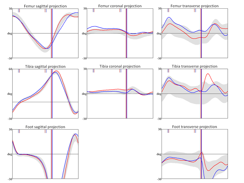
The rockers provide mechanisms for the tibia to move forward over the foot and hence for the passenger unit to be carried forward in stance. If we look at the angle the tibia makes to the vertical (above) then we can see that it starts off about 20° behind vertical at foot contact and progresses forwards reasonably steadily (with a bit of a wobble) to reach about 50° in front of vertical at foot off.

tibial progression

Perry explains this in terms of three rockers.  Early on the whole foot rotates about the heel. Later on the tibia rotates over the foot about the ankle and then finally the whole foot rotates about the forefoot (see below). Easy eh!

rockers

There is no doubt that all three mechanisms make important contributions to tibial progression. I’m not quite so convinced by Perry’s implication that these occur as a sequence of discrete mechanisms. To investigate this we need to look at the dorsiflexion graph which tells us when ankle rocker occurs and the foot projections graph that tells us when the heel and forefoot rockers are active (see graphs below, note that is impossible to distinguish the timing of the rockers from the ankle angle graph alone ).

Rocker graphs


Heel rocker starts off at foot contact and proceeds until the foot is flat at about 8% of the gait cycle (in red above). It should be noted that this is considerably longer than the period to maximum plantarflexion in early stance that it is sometimes related to. Ankle rocker is the period over which the dorsiflexion angle increases which we can see from the ankle angle graph is from about 5% of the gait cycle to about 45%. There is thus a short period of overlap when both the heel and ankle rockers are active.

Forefoot rocker starts with heel lift which Perry suggests occurs at mid-stance (30% gait cycle). The data depicted above suggests it might commence even earlier (20%?) and it continues until the end of stance. It is thus clear that there is a considerable period from about 20% of the gait cycle until 45% when both ankle and forefoot rockers and simultaneously active.

The conclusion is that whilst the rockers are undoubtedly the mechanisms which allow the tibia to progress they form an overlapping progression rather than a series of discrete events. Indeed for the majority of stance two rockers are active simultaneously.

Since Perry introduced the concepts there has been some slippage in how the terms have been applied which is best avoided. As far as I can see, Perry always talked about heel, ankle and forefoot rockers and never first, second and third rockers. I think this is good practice as quite a lot of our patients don’t have a first rocker (they make contact with the forefoot rather than the heel). It’s always seemed a little illogical to me for someone to have a second rocker if they’ve never had a first rocker!

The other common misconception is that the rockers are alternative labels for phases of the gait cycle. Again Perry never used them in this sense, for her they are mechanisms that allow the tibia to move forward over the foot not phases of the gait cycle. It is particularly erroneous to apply these terms to phases of pathological gait. Many kids with CP never make heel contact and it is thus completely inappropriate to refer to early stance as the phase of heel rocker.

This reinforces the fact that the rockers are mechanisms of normal gait and great care is required in applying the terms to walking with pathology. If a child with CP makes contact with the toe after which the foot comes flat later in stance then they must use a mechanism that might best be described as a reverse forefoot rocker during which the heel is being lowered to the ground rather than being raised. Similarly if they employ a vault to assist clearance of the swing limb then they will often have a reversed ankle rocker during which plantarflexion (rather than dorsiflexion) increases.

Referring back to the work I described in my blog the week before last strongly suggests to me that, in bare feet, the heel rocker is actually a heel roller with the movement being a rolling on the curved surface of the posterior-distal calcaneus rather than a pivot about a particular point on the heel. On the other hand if walking in a shoe with a reasonably stiff heel it is more likely that a rocker like mechanism does occur. The appropriateness of this terminology may thus depend on footwear as well as gait pathology.

PS. In the second edition of Gait AnalysisPerry and Burnfield describe a fourth toe rocker very late in stance.  This can certainly be seen on slow motion videos but I’m not aware of any detailed studies of its biomechanical significance. It looks to occur very late on and I suspect only after most of the load has been taken off the foot but it would be nice to see a more definitive analysis of this.

Projection angles

I’ve had some feedback from Vicon support that people have been asking them how to calculate what I’ve called projection angles on page 138 of my book. These are graphs that look a bit like joint kinematics but represent how each of the segments is aligned with respect to the global axis system rather than to the proximal segment. Two of the femur projection angels thus show how the long axis of the femur is tilted with respect to the vertical in the global sagittal and coronal planes. The third angle shows how the femur is rotated about this axis (projected onto the transverse plane).

projection angles


I first plotted these graphs as a quality assurance tool in that they represent what you should see on  a video recording of the person walking (as long as you take into account parallax effects if the person is not in the centre of the screen or the camera is not directed exactly along one of the principal axes of the global coordinate system). Thus the femur transverse projection tells you whether you should be seeing the femur as internally or externally rotated as viewed by a camera towards which the person is walking. It avoids the need to perform a mental sum of pelvic rotation and hip rotation to assess which is required otherwise. In the example above, at foot contact the left thigh (red) is facing directly ahead and the right thigh is internally rotated by about 5°. You probably won’t be see such a small difference but if the right limb looked to be externally rotated at this instant you might want to question the alignment of thigh markers or knee alignment devices.

Since starting to plot the angles, however, a range of other uses have emerged. The tibia and femur sagittal projections, for example, are essentially what Elaine Owen refers to as segment to vertical angles when tuning ankle foot orthoses.

The foot transverse plane angle is what many of us already plot out routinely and call foot progression. The corresponding angle in the sagittal plane, however, is very rarely plotted but gives a direct appreciation of whether the foot is flat or not. In the example above the foot makes contact at an angle of about 15° to the ground and rotates to become flat on the floor (0°) during about the first 8% of the gait cycle (Perry’s heel rocker). It then remains flat until about 40% of the gait cycle (ankle rocker) after which heel rise causes the foot to start tilting forwards (negative angle, representing toe rocker). If distinguishing between the rockers is important to you then using a graph like this is about the only way to do it. I’ve referred in a previous post to how useful I find this information can be.

I’ve not plotted the pelvic graphs because, if you calculate them using the correct rotation sequence, then they are virtually identical to the pelvic joint angles.

The main reason for this post is thus to make the model that I wrote many years ago to calculate this widely available (click here to go to the download page). Unfortunately it is written in Vicon’s BodyLanguage so will only be directly useful for Vicon users (please note that it requires plugin Gait to have been run first). The accompanying description of exactly what the angles represent should, however, allow any reasonably competent clinical engineer to calculate the equivalents in any other programming/modelling language.

Is it all just too bloody complicated?

I’ve just got back from the ESMAC-SIAMOC meeting in Rome. We’ve been entertained royally for three days in the aulas and cloisters of the Thomas Aquinus University. It has once more been a fantastic opportunity to network and exchange ideas and on one level I come back rejuvenated and inspired.

I say “on one level” because on another level I’ve also come back somewhat disappointed – disappointed because there was little in the scientific programme which left me feeling I understood things better than I did before I arrived. A large number of papers could be summed up by the conclusion, “we understand this area less after performing this research than we did before we started”.  I don’t think it is just ESMAC-SIAMC that suffers in this way. I see it at most of the conferences I attend and in a lot of papers that I read (and, if I’m being honest, in some of the papers that I write).

Just two areas illustrate this. One is in the advanced and complex modelling that is so often the focus of contemporary biomechanics. We learnt (or had confirmed) in Rome that the results are highly dependent on the details of how the individual anatomy is parameterised and of the calibration processes used to define joint centres.  The overall conclusion is that we are less confident in the output of our simulations and models after we’ve performed this research than we were before. Of course it is important to know what the limitations of our research. At some stage, however, we will have to acknowledge those limitations and accept the conclusion that the biological complexity of the human neuromusculoskeletal system is just too great for us to stand any chance of applying these techniques usefully (at least not beyond the constraints of healthy people exercising tightly controlled tasks).

The other field is that of measuring spasticity. Seven or eight years ago I was really excited about the prospect of instrumenting clinical tests to quantify spasticity more rigorously. The results I’ve seen reported are really quite disappointing in that it seems that spasticity is a rather complex and badly behaved phenomenon that simply refuses to be measured.  I have little faith any longer that spasticity is a purely velocity dependent response  (Lance, 1980) and the additional complexity that is introduced when displacement, acceleration or even jerk might have to be considered removes any hope that we will ever understand how these components interrelate within the current paradigm.

One of the “advantages” of research leaving us less clear of what is happening than we were before is that it opens up the conclusion that “further research is required to better understand these phenomena”. Research thus begets research and the university departments rub their hands in glee at the prospect of more research grants, papers and citations. For many of us it leads to increased job security. We have a vicious circle that delights and thrives in creating complexity and chaos.

This is particularly bizarre in orthopaedic and rehabilitation fields (and perhaps more widely across health sciences) in that the tools we have to treat our patients are generally extremely blunt. Selective dorsal rhizotomy, intrathecal baclofen and botulinum toxin are the only tools we have to manage spasticity. At a clinical level the only decision we need to make is which, if any, of these to use. If we want our research to be clinically useful we need to concentrate on the simple questions that need to be answered before we turn our focus to the more complicated ones that don’t.

The small number of presentations that did impress me posed a research question in such a way that the answer actually improved my understanding of a given issue. Almost all of these resulted in me having a clearer, simpler view of the world after the presentation. This doesn’t necessarily require simplistic techniques. The walk-DMC scale that Kat Steele and Mike Schwartz proposed in their prize winning paper (page 25 of Abstract Book) uses a sophisticated technique. It is a technique, however, that has been appropriately selected to answer a well posed research question (Can we quantify the effect of disordered motor control on walking in children with cerebral palsy?). Once the appropriate techniques has been selected the answer is simple (Yes, at least on the basis of the preliminary analysis they presented).

One of the most ancient tests of the scientific quality is Occam’s Razor, that science (and our thinking in general) should be as simple possible but no simpler. It would be interesting to perform an audit of the presentations at any contemporary conference against this criterion. I suspect the results would be quite sobering.

.

Lance, J. (1980). Pathophysiology of spasticity and clinical experience with baclofen. In R. Feldman, R. Young & W. Koella (Eds.), Spasticity: disordered motor control (pp. 485-495). Chicago: Year book medical publishers.

What is normal?

A couple of months ago I wrote a post entitled normative data capture Part 1. No-one has yet demanded Part II but I’ll give it anyway. The earlier post concentrated on what sort of numbers were required to determine normative ranges for any data assuming we want a reasonable estimate of both the average and the standard deviation.

Once we’ve got the numbers sorted out then the question arises “What is normal?” It might be worth starting with a paragraph addressing the political dimension here. The word “normal” is considered inappropriate in some circles because of the connotation that anyone else, our patient for example, is “abnormal” which is considered a negative term. The response from some researchers (particularly Americans?) working with children has thus been to prefer the term typically developing. This presumable implies that our patients our atypical and I’m not sure that that is any better or worse than abnormal.  What I do appreciate is that we are all abnormal in some regard. The question should not be whether the person is normal or abnormal but whether their gait pattern is. I think normative stresses this emphasis that it is the data or the pattern that is abnormal rather than the individual (but others may think differently).

But then what is a normal gait pattern?  In my dictionary there are various definitions of normal and the closest to the sense in which we are using it is not deviating from the standard. Even this though is not particularly close. I suspect that what we really mean is representative of the population. This raises the questions of how we consider people, with conditions such as  cerebral palsy  in relation to this population?  I think that conceptually they should be considered as part of the population. Thus the normal population includes people with cerebral palsy (and other gait disorders). In childhood and early adulthood at least, these conditions are quite rare (approximately 1 in 500 people is born with CP, one of the more common conditions affecting walking) so true normative ranges (calculated over a wide enough sample) would be very little affected by including or excluding them.

Of course we most often collect normative data from much smaller samples (my previous post suggested that 30 might be regarded as a reasonable number). In this case it makes sense to specifically exclude people with obvious neuromusculoskeletal pathology not because we regard them as abnormal in principle but because the statistics of the situation dictate that the normative data that we obtain by excluding them will be closer to normative data for the entire population than the data we would obtain if they were included. (Including one person with CP in a sample of 30 runs the risk of obtaining normative data that is quite different from that which would result from the one person in 500 in the general population)

A more common problem is a number of anatomical and physiological characteristics which have a wide range within the general population such as in and out-toeing, tibial torsion, femoral anteversion, flat-feet and high arches. Some health professionals will want to define an arbitrary and often subjective cut-off beyond which the individual is labelled as having an impairment and exclude them from the normative dataset. I remember hearing one story of a gait analysis service that was interested in providing normative data for a foot model and simply collected a group of individuals who, to them, had no obvious neuromusculoskeletal impairment and were entirely asymptomatic. The team was later joined by another health professional who looked at the dataset and concluded that quite a large proportion of the cohort had either flat feet or raised arches and wanted these abnormal people deleted from the dataset.

This of course raises the prospect of self-fulfilling prophecy. People with flat feet are considered as abnormal because they have data that falls outside the range of those who have been assessed as not having flat feet. This is clearly daft. Normative data ranges should ideally be generated with randomly sampled datasets from the whole population. In practical situations random sampling is extremely rare but it is inappropriate to select participants on the basis of some pre-supposition of what normal is (unless the abnormality is so rare and severe that the inclusion in a small sample risks skewing the data as described above).

There is another problem when we start to look at older populations. Iezzoni et al. (2001) suggest that over 10% of the entire population have some difficulty walking as little as 400m, rising to nearly 50% if we look at the population aged 80 and over. There is considerably potential for inclusion or exclusion of these individuals to affect normative data. If we are concerned with what data to use for comparative purposes in older populations, however, then I think the goal posts have shifted.  What we really require is not normative reference data but reference data from healthy people within a particular age range or more specifically those without any specific neuromusculoskeletal pathology. If we want a convenient shorthand then perhaps we should refer to a healthy gait pattern in these circumstances rather than a normal one.

There are the same risks here of subjective decisions as to where the healthy range ends and pathology starts which are largely unavoidable. These can be addressed to a certain extent by defining explicit and objective inclusion criteria. We might not agree with definitions but at least we will know what they are. Even these are problematic however because it is very easy to introduce sampling bias when recruiting. When selecting healthy controls for a study there will be a tendency to select the healthiest available.  All will fulfil the inclusion criteria but they may not be representative of the population of all people who fulfil those criteria.  The solution here may be to specify the characteristics of the sample that were actually recruited rather than the inclusion criteria for the study.

.

Iezzoni, L. I., McCarthy, E. P., Davis, R. B., & Siebens, H. (2001). Mobility difficulties are not only a problem of old age. Journal of General Internal Medicine, 16(4), 235-243.

Do it yourself normative data comparison (free download!)

Hi, I’ve had a bit of a break over the summer but I’m hoping to start posting again regularly form now on. Just a reminder that we are running another gait course in November (this one focussing on measurement issues rather than clinical interpretation). Click on the image to the right for more details. There is also just about time to register to start our Masters in Clinical Gait Analysis by distance learning (you don’t need to come to Salford at all). Click on the other image to the right for more details of it.

Enough of the ads, this blog following on from one I wrote just after the GCMAS meeting last year. It had a video link to the presentation I’d just delivered arguing that the reason we collect normative data should be so that we can compare it with other people’s normative data. I presented data showing that if we did that for the normative data from the Royal Children’s Hospital in Melbourne and Gillette Children’s Speciality Healthcare then we get quite remarkable agreement. You can see the comparative kinematic data in the figure below.

compare norms

The paper based on that presentation has finally got published in Gait and Posture (if you don’t have access to the journal you can find a pre-publication version here). We’ve also prepared an Excel file that contains the data in a format that allows you to add your own normative data (mean and standard deviation) to allow comparison with the data from Melbourne and Gillette. Just cut and paste your data into the spreadsheet and look at the graphs to see how you compare. Remember that differences in the mean traces suggest that there are systematic differences in how you apply markers, differences in standard deviations are likely to reflect how consistently you apply them within your own lab.

Do let me know how well your data compares. It might be interesting to post some examples of how various clinical centres compare on this blog-site somewhere.