Why do we collect normative data?

The sun is still shining in Cincinnati although many of us in the conference hotel are seeing very little of it. Thought I’d share the podium presentation I’ve just made which reflects on why it is that we collect service specific normative reference data. It’s my feeling  that this should be to allow us to compare data between services in order to develop consistent practices rather than as a way to allow us to continue to tolerate differences in the way different services make measurements. Anyway if you want to you can listen to the screen cast below.

There was an interesting technical extension to the work which I was unable to include in the presentation because of tht time limit. This is covered in the screen cast below.

Mind your language

I’m here in Cincinnati for the Gait and Clinical Movement Analysis Society Annual Meeting. Lovely sunshine makes a change from damp old Manchester.

Anyway today was pre-conference tutorial day and started with a really interesting session with  Art Kuo trying to help us understand induced acceleration analysis. He was particularly concerned to try and demystify the subject using a number of worked examples to show it is possible to get a qualitative feel for the accelerating effect that different joint torques will have on different segments.  He used these to help us understand the sometimes counter-intuitive conclusions that these analyses can lead us to. I found the approach fascinating and will go away and work through some examples myself. I’ll need to think a bit more before I commit any reflections to this blog.

Right at the end he volunteered some fascinating thoughts on terminology that I think are worth passing on immediately. He commented on how some of the terminology we use for accelerations tends to have inappropriate positive and negative connotations and that we need to be very careful that this doesn’t lead us to inappropriate conclusions.

One pair of phrases was “propulsion” and “braking”. We tend to think that propulsion is good and braking is bad but in cyclic walking this is not the case. If  we haven’t changed our speed over a complete gait cycle then, following Newton’s laws, we will have propulsive and braking forces that match exactly (or  more technically propulsive and braking impulses match). All that increasing the propulsive forces does is require an increased demand for braking forces to be applied. To understand how we walk the way we do we really need to have a more nuanced understanding of why braking and propulsive forces are required at all. I agree with Art that using words that suggest that one is beneficial and the other detrimental is not useful.

The other pair was “support” and “falling” (or equivalent ). Again joint torques that apply an upwards (supporting) force to the centre of mass are generally considered to be good whereas those that accelerate the body downwards are considered bad. Again, however, if walking is cyclic then there is no net acceleration of the centre of mass in either direction. I’m less sold on this argument as there is a requirement for the upward forces to average bodyweight over the gait cycle and thus I think there is a sense in which the support mechanisms are more important than those that allow downward accelerations – but I do agree with Art again that if the body accelerates upwards in one part of the gait cycle it must fall in another. Considering one of these as good and the other as bad is not likely to help our understanding.

What Art didn’t propose was alternative words that don’t have these associations. Anyone any ideas?

Stretching time

Here’s something I’ve meant to share for some time.

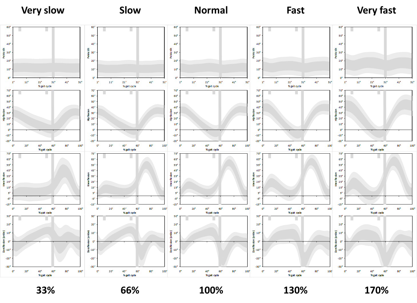
Below are two graphs that I prepared for some teaching I was doing in Melbourne last August. I downloaded the data that Mike Schwartz has been so kind as to make available from his study looking at the changes in gait pattern of children when they walk at different speeds (Schwartz et al., 2008). I then formatted the sagittal plane graphs as we normally do (except that I’ve started plotting the two standard deviation range in a different shade of grey to the one standard deviation range to remind us that we often under-estimate the spread of our reference data). Data is time normalised to the gait cycle and plotted on graphs of fixed aspect ratio (3:4 in this case). All looks quite unremarkable with fairly modest changes in kinematics with walking speed.

Different speeds time normalised

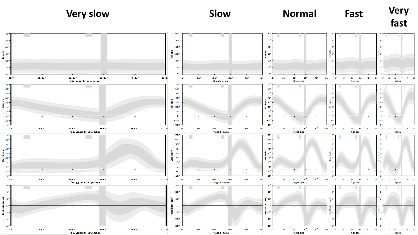
But then I realised that the slower walkers have a longer cycle time and the data should really be stretched to make comparisons as to how children are waking in real time. Slow walkers take a lot longer to complete a gait cycle than fast walkers and the data should really be plotted on wider graphs to allow comparison of  what is happening over the same time period.

Different speeds not time normalised

If we plot the data like this we see just how different the data really are. I’ve not absorbed the full effect or implications of this but think about the slope of the knee flexion curve in second double support and toe off which many clinicians associate with rectus femoris (mal)function. If the rectus is inhibiting knee flexion then they expect the slope to be reduced.  But look at the difference between the real gradient in the lower graphs and the apparent gradient in the conventional (upper graphs). How can we possibly interpret this phenomenon from the conventional graphs?

It ‘s not clear what we can do about this. Plotting the graphs the way we do allows comparison of like with like (even if we might lose something by forcing the comparison). We often use graphs to compare outcome after intervention. How would we do this sensibly if the graphs are different shapes?

Anyone got any ideas how we can properly represent the slope data without losing the power of the straight forward comparisons we get from sticking to the tried and tested conventions for plotting data?

.

Schwartz, M. H., Rozumalski, A., & Trost, J. P. (2008). The effect of walking speed on the gait of typically developing children. J Biomech, 41(8), 1639-1650.

Making nice gait graphs in Excel

This is quite a simple post with a tutorial screencast of how to format gait graphs nicely in Excel. For a long time I just didn’t think this was possible but you can see from the image below that it is! The screencast is the simplest example of a range of tools we are developing to support students who enrol on ourmaster’s degree programme in clinical gait analysis which starts in September as part of the EU funded CMAster project.

Nice gait graph

The main thing that makes plotting the graphs like this possible is that you can select different series within the same chart to have different chart types. I suspect that this feature may not be available in early versions of Excel but don’t know when it was introduced – this graph was generated in Excel 2010 on a PC. If you are good at working with charts in Excel then this is all you really need to know and watching the screencast will only waste another 20 minutes of your life. If you are not then I suggest you just watch the screencast and I’ll explain things a bit more slowly.

One top tip I’ll offer – if you want to create an array of graphs make sure that your formatting is correct on the first graph before you start copying and pasting. If you find a mistake later on you’ll have to correct it on each graph separately.

I’ve said in the screencast that I’ll produce another one to show how to add in the timing data. The only way I know to do this is a little bit messy. Does anyone know a nice straightforward way?

(Note that the screencast is recorded in reasonably high definition but you may have to use full screen display and increase the resolution with the little cog icon at the bottom left of the video to appreciate this.)

Where’s the foot?

foot pitch

Another comment from CMAS. I think it was Alison Richardson who was presenting at one point and remarked, “but of course we can’t tell where the foot is from the graphs”. How true? and why not? Conventionally in clinical gait analysis we plot where the pelvis is in relation to the lab, then the hip, knee and ankle joints. In theory if you know all this information you can work out the orientation of the foot. I don’t know anyone, however, who has developed the knack of adding all those angles up in their head to work this out. In understanding how the foot is contributing to that pattern I think Perry’s concept of foot rockers is key – is the limb pivoting primarily around the heel, the ankle or the MTP joint? Yet, despite what you hear in many discussions about gait data, it’s virtually impossible to tell from the graphs which rocker is active at  any given time.

So why don’t we plot out foot orientation? We calculate the equivalent in the transverse plane and call it foot progression. I think it would make all our lives considerably easier if we added an extra graph at the foot of the sagittal plane data. Given that the pitch of a shoe is how much it tilts the foot forwards perhaps we should refer to this a “foot pitch”.

I’ve shown you what the sagittal graphs would then look like. I don’t suggest using the colours on the foot pitch graph – they are only there to show you how easily you can pick out the three rockers. During the red phase of stance the foot is pivoting about the heel – first rocker. During the white phase the foot is flat on the ground – second rocker. During the blue phase the foot is pivoting about the MTP joint (or toe) – third rocker (or third and fourth rockers if you want to use Perry and Burnfield’s most recent terminology (2010). Notice that end of first rocker does not coincide with opposite foot off but is completed appreciably earlier. Many people don’t appreciate just how early third rocker starts either.
.

.
Perry, J., & Burnfield, J. M. (2010). Gait analysis: normal and pathological function (2nd ed.). Pomona, California: Slack.